Digital Signal Processing (DSP): How It Works, Components, Techniques, and Applications
You’ll learn what Digital Signal Processing (DSP) is and how signals become useful digital data. It shows how signals are captured, filtered, sampled, processed, and turned back into usable outputs. You’ll also see the main system parts, common DSP techniques, key performance parameters, and typical applications. Finally, it compares DSP with analog signal processing so you know when each is used.Catalog
Figure 1. Digital Signal Processing (DSP)
What is Digital Signal Processing (DSP)?
Digital Signal Processing (DSP) is the method of analyzing and modifying signals in digital form, whether they originate from measurements or already-digital sources. Physical signals such as sound, temperature, vibration, voltage, images, and radio waves are often converted into analog electrical signals by sensors and then digitized by an analog-to-digital converter (ADC), although some sensors provide digital outputs directly. Once in numeric form, a processor mathematically filters noise, extracts information, enhances quality, or compresses data before sending it to storage, display, or communication systems. DSP allows electronic systems to mathematically analyze, transform, and reconstruct signals using numerical algorithms instead of purely analog circuits.
How Digital Signal Processing Works?
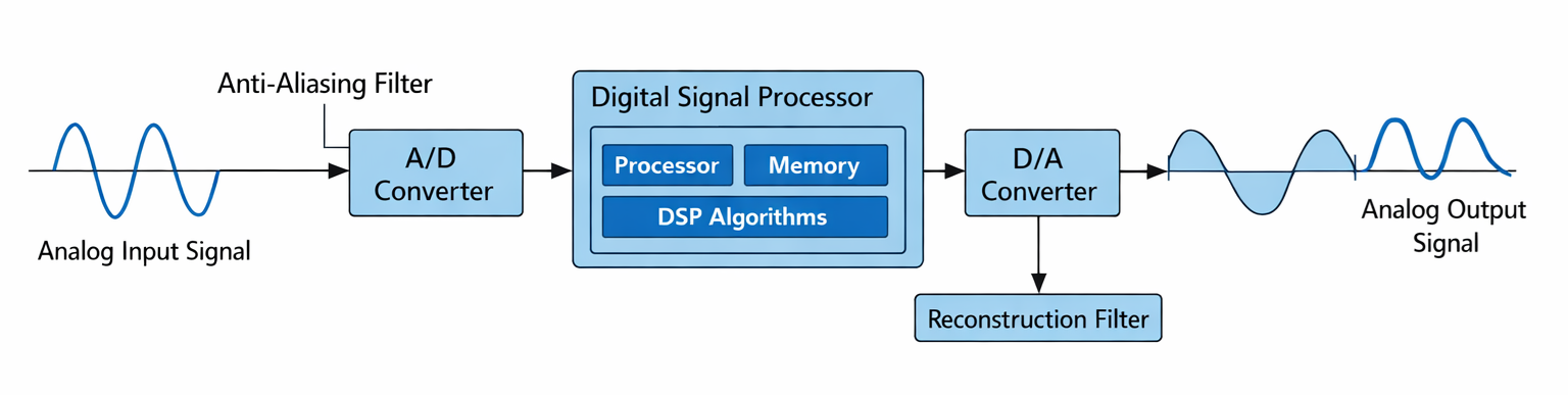
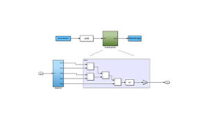
Figure 2. DSP Working Principle
A typical DSP measurement system operates in a sequence that converts a signal into digital form for computation, although some DSP systems process already-digital data and do not require analog conversion. As shown in the diagram, the process begins with an analog input signal produced by a sensor such as a microphone, antenna, or measuring device. Before digitization, the signal passes through an anti-aliasing filter that restricts the signal bandwidth to less than half the sampling frequency to prevent aliasing distortion. The conditioned waveform then enters the A/D converter (ADC), where it is sampled at discrete time intervals and quantized into discrete amplitude levels, producing a binary digital representation.
The digital data is then processed by a processing system such as a DSP chip, microcontroller, CPU, GPU, or FPGA running DSP algorithms that perform mathematical operations such as filtering, transformation, and detection. After processing, the digital output is sent to the D/A converter (DAC) to recreate an analog signal. Because the DAC produces a staircase (zero-order hold) approximation of the waveform, it passes through a reconstruction filter that smooths the waveform, producing a smoothed band-limited analog approximation of the original signal.
Components of a DSP System
|
Component |
Function |
|
Sensor /
Transducer |
Converts a
physical quantity into an electrical or digital signal |
|
Analog
Front-End |
Performs
signal conditioning such as amplification, impedance matching, level
shifting, and protection |
|
Anti-Aliasing
Filter |
Restricts
signal bandwidth to less than half the sampling frequency to prevent aliasing |
|
ADC |
Samples and
quantizes the analog signal into digital data |
|
DSP Processor |
Executes DSP
algorithms and mathematical operations on digital data |
|
Memory |
Stores
programs, coefficients, intermediate buffers, and input/output data |
|
DAC |
Converts
digital data to a staircase analog signal that typically requires
reconstruction filtering |
|
Output Device |
Analog
actuator, display, storage system, or digital communication interface |
Types of Digital Signal Processing Techniques
Filtering Techniques
Filtering is the process of removing unwanted parts of a signal while keeping useful information. The noisy waveform enters the digital filter and a cleaner waveform appears at the output. FIR filters work using only present and past input values, which makes them stable and predictable. IIR filters reuse previous outputs to create sharper filtering with fewer computations. Because of this feedback behavior, IIR filters must be carefully designed to avoid instability. These digital filtering methods are commonly used for noise removal in audio signals and sensor measurements.
Transform Techniques
Transform processing changes a signal into another mathematical form so its characteristics are easier to observe. The waveform is converted from time variation into another representation showing hidden details. The FFT reveals the signal’s frequency components clearly. The DCT groups signal energy efficiently for multimedia compression systems. The Wavelet transform shows both short and long signal features at different scales. These transforms are used to study signals in communication and media applications.
Spectral Analysis
Spectral analysis examines how signal energy spreads across frequencies. A waveform is converted into a spectrum containing peaks at specific frequencies. From this view, harmonics and bandwidth can be measured directly. Dominant tones become visible even when they are hard to notice in the original waveform. This method is useful for vibration diagnostics and radio signal inspection. It helps determine whether a signal behaves normally or contains abnormal components.
Adaptive Processing
Adaptive processing automatically adjusts system behavior based on incoming data. The output error feeds back into the system to refine its response. The algorithm continuously updates internal parameters to match changing conditions. This allows the system to track noise or interference over time. It is commonly used in echo cancellation and background noise suppression. The result is a cleaner and more stable signal in dynamic environments.
Compression Processing
Compression processing reduces the size of digital data while preserving important information. A large data stream becomes a smaller encoded stream after processing. Redundant patterns are removed and less noticeable details may be simplified. This reduces storage requirements and transmission bandwidth. Audio, image, and video formats rely heavily on this technique. It allows faster communication and efficient data handling in multimedia systems.
Technical Specifications of DSP
|
Parameter |
Numeric Range |
|
Sampling Rate |
8 kHz
(speech), 44.1 kHz (audio), 96 kHz–1 MHz (instrumentation) |
|
Resolution
(Bit Depth) |
8-bit,
12-bit, 16-bit, 24-bit, 32-bit float |
|
Processing
Speed |
50 MIPS –
2000+ MIPS or 100 MMAC/s – 20 GMAC/s |
|
Dynamic Range |
~48 dB
(8-bit), 72 dB (12-bit), 96 dB (16-bit), 144 dB (24-bit) |
|
Latency |
<1 ms
(control), 2–10 ms (audio), >50 ms (streaming acceptable) |
|
Signal-to-Noise
Ratio (SNR) |
60 dB–140 dB
depending on converter quality |
|
Memory
Capacity |
32 KB – 8 MB
on-chip RAM, external memory up to GB |
|
Power
Consumption |
10 mW
(portable) – 5 W (high-performance DSP) |
|
Word Length |
16-bit fixed,
24-bit fixed, 32-bit floating point |
|
Clock
Frequency |
50 MHz – 1.5
GHz |
|
Throughput |
1–500
Msamples/s |
|
Interface
Bandwidth |
1 Mbps – 10
Gbps (SPI, I2S, PCIe, Ethernet) |
|
ADC Accuracy |
±0.5 LSB to
±4 LSB |
|
DAC
Resolution |
10-bit –
24-bit |
|
Operating
Temperature |
−40°C to
+125°C (industrial grade) |
Applications of DSP
Digital signal processing is used to measure, improve, and analyze signals automatically, including the following applications:
• Audio processing (noise suppression, echo cancellation, equalizers)
• Speech recognition and voice assistants
• Image processing in digital cameras (demosaicing, filtering, enhancement, and compression)
• Biomedical signal monitoring (ECG, EEG) and medical imaging (ultrasound)
• Wireless communication systems (modulation, demodulation, channel coding, synchronization, and equalization)
• Radar and sonar detection
• Industrial vibration monitoring
• Power system protection and harmonic analysis
• Motor control and automation feedback systems
• Video compression and streaming codecs
DSP vs Analog Signal Processing
|
Feature |
Digital
Signal Processing |
Analog
Signal Processing |
|
Signal
Representation |
Sampled
values at discrete time steps (e.g., 44.1 kHz sampling) |
Continuous
voltage/current waveform |
|
Amplitude
Precision |
Quantized
levels (e.g., 2¹⁶ = 65,536 levels at 16-bit) |
Continuous
but limited by component accuracy (±1–5%) |
|
Frequency
Accuracy |
Exact
numerical frequency ratios |
Drift depends
on RC/LC tolerances and temperature |
|
Repeatability |
Identical
output for same data and code |
Varies
between units and over time |
|
Noise
Susceptibility |
Only
front-end affected after conversion |
Noise
accumulates through entire circuit path |
|
Temperature
Stability |
Minimal
change (digital logic threshold based) |
Gain and
offset vary with °C coefficient of components |
|
Calibration
Requirement |
Usually
one-time or none |
Often
requires periodic recalibration |
|
Modification
Method |
Firmware/software
update |
Hardware
redesign required |
|
Long-Term
Drift |
Limited to
clock accuracy (ppm level) |
Component
aging causes %-level drift |
|
Mathematical
Operations |
Precise
arithmetic (add, multiply, FFT) |
Approximate
using circuit behavior |
|
Dynamic
Reconfiguration |
Real-time
algorithm switching possible |
Fixed
topology |
|
Delay
Behavior |
Predictable
processing delay (µs–ms) |
Near-instant
but varies with phase shift |
|
Scalability |
Complexity
increases by computation |
Complexity
increases by added components |
|
Integration
Level |
Single chip
can replace many circuits |
Requires
multiple discrete components |
|
Typical
Applications |
Modems, audio
processing, image processing, control logic |
RF
amplification, analog filtering, power amplification |
Conclusion
DSP converts signals into discrete data so they can be filtered, transformed, detected, compressed, and interpreted using mathematical algorithms. System performance depends on sampling rate, resolution, processing speed, dynamic range, latency, and noise behavior. Its flexibility and stability make it suitable for communications, multimedia, control, medical monitoring, and industrial analysis, while analog processing remains useful for simple or extremely low-latency tasks. Together, both approaches complement each other in modern electronic systems.
About us
ALLELCO LIMITED
Read more
Quick inquiry
Please send an inquiry, we will respond immediately.
Frequently Asked Questions [FAQ]
1. Do I need a dedicated DSP chip or can a microcontroller handle DSP tasks?
For simple filtering, sensing, or control, a standard microcontroller is usually enough. A dedicated DSP processor is recommended when you need fast real-time processing such as audio effects, vibration analysis, or wireless communication decoding.
2. Is floating-point DSP better than fixed-point DSP?
Floating-point DSP is easier to program and handles large dynamic ranges, making it ideal for audio and scientific measurements. Fixed-point DSP is cheaper, faster, and more power-efficient, which suits embedded and battery-powered devices.
3. Can DSP improve sensor accuracy in industrial environments?
Yes. DSP can remove electrical noise, vibration interference, and measurement spikes, allowing sensors to produce more stable and reliable readings even in harsh environments.
4. Does DSP increase power consumption in embedded devices?
It can, but modern low-power DSP chips are optimized for efficiency. Using optimized algorithms and sleep modes keeps battery usage low in portable equipment.
5. How do I choose between FPGA-based DSP and processor-based DSP?
Choose processor-based DSP for flexibility and easier programming. Choose FPGA-based DSP when you need ultra-high speed parallel processing such as video processing, high-frequency communication, or radar systems.
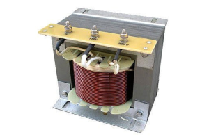
Understanding Shell Type Transformers
on February 12th
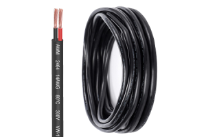
14 AWG Wire Explained: Size, Ampacity, Breaker, and Uses
on February 11th
Popular Posts
-

Complex Instruction Set Computers: How They Changed Computing?
on April 18th 147749
-

USB-C Pinout and Features
on April 18th 111908
-
Using Xilinx Unified Simulation Primitives: A Comprehensive Guide to FPGA Design and Simulation
on April 18th 111349
-

Power Supply Voltages in Electronics: Meaning of VCC, VDD, VEE, VSS, and GND
on April 18th 83714
-

RJ45 Connector Guide: Pinout, Wiring, Cable Types, and Uses
on January 1th 79502
-

The Ultimate Guide to Wire Color Codes in Modern Electrical Systems
The way our electrical systems use colors isn’t just for looks. Each wire color now indicates a specific function, making it easier to identify and handle electrical components correctly during ins...on January 1th 66869
-

Quality (Q) Factor: Equations and Applications
The quality factor, or 'Q', is important when checking how well inductors and resonators work in electronic systems that use radio frequencies (RF). 'Q' measures how well a circuit minimizes energy...on January 1th 63004
-
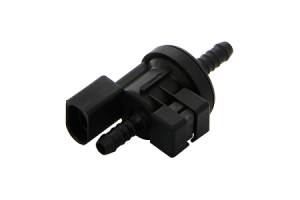
Purge Valve Guide: Function, Symptoms, Testing, and Replacement for Optimal Engine Performance
The purge valve is a key part of a car’s system that helps keep the air clean by managing fuel vapors before they can escape into the atmosphere. This not only helps the environment by reducing pol...on January 1th 62947
-

Achieving Peak Performance with the Maximum Power Transfer Theorem
The Maximum Power Transfer Theorem explains how energy from a source, such as a battery or generator, flows to a connected load. It shows the exact condition where the load receives the most power....on January 1th 54077
-

A23 Battery Specifications and Compatibility
The A23 battery is a small, cylinder-shaped battery with high voltage. Also called 23A, 23AE, or MN21, it runs at 12 volts and much higher than AA or AAA batteries. Its special design make...on January 1th 52089
HOT Part Number
-

BD9B100MUV-E2
Rohm Semiconductor
IC REG BUCK ADJ 1A 16VQFN
UPD70F3539AF5A9-PN7-Q-A
Renesas Electronics America Inc
IC MICROCONTROLLER
18081A621JAT2A
KYOCERA AVX
CAP CER 620PF 100V NP0 1808
FDN340P
onsemi
MOSFET P-CH 20V 2A SUPERSOT3
70231-101
Amphenol ICC (FCI)
CONN RCPT BLADE PWR 8POS EDGE MT
MPSW42RLRAG
onsemi
TRANS NPN 300V 0.5A TO92
MC7824BT
onsemi
IC REG LINEAR 24V 1A TO220AB
AD8009ARZ-REEL
Analog Devices Inc.
IC OPAMP CFA 1 CIRCUIT 8SOIC
LT1815CS5#TRPBF
Analog Devices Inc.
IC OPAMP VFB 1 CIRCUIT TSOT23-5
DG411DYZ
Renesas Electronics America Inc
IC SWITCH SPST-NCX4 35OHM 16SOIC
VFT2060C-M3/4W
Vishay General Semiconductor - Diodes Division
DIODE SCHOTTKY 20A 60V ITO-220AB
TSX562AIYST
STMicroelectronics
IC CMOS 2 CIRCUIT 8MINISO
MR256D08BMA45
Everspin Technologies Inc.
IC RAM 256KBIT PARALLEL 48FBGA
VSC3312YYP-01
Microchip Technology
IC SWITCH 16X16 6.5GBPS 196FCBGA
XC68HC908GP20CFB
Motorola
TSG 8BIT20K FLASH
CSR8811A08-ICXR-R
Qualcomm
IC RF TXRX+MCU BLUETOOTH
MPSW05
onsemi
TRANS NPN 60V 0.5A TO92
1N4055R
Solid State Inc.
DIODE GEN PURP REV 900V 275A DO9 -

ASX342ATSC00XPED0-DP
onsemi
IMAGE SENSOR VGA 1/4 CIS SOC
0433.125NR
Littelfuse Inc.
FUSE BOARD MNT 125MA 125VAC/VDC
1SMA5941BT3G
onsemi
DIODE ZENER 47V 1.5W SMA
DCP010512BP-U/700
Texas Instruments
DC DC CONVERTER 12V 1W
1-1734344-1
TE Connectivity AMP Connectors
CONN D-SUB HD RCPT 15P R/A SLDR
KSD1621STF
onsemi
TRANS NPN 25V 2A SOT89-3
BQ24161RGET
Texas Instruments
IC BATT CHG LI-ION 1CELL 24VQFN
BTA26-600BW
STMicroelectronics
TRIAC ALTERNISTOR 600V 25A TOP3
NCP1239DD65R2G
onsemi
IC OFFLINE SWITCH FLYBACK 7SOIC
TMS320TCI6482BZTZA
Texas Instruments
TMS320 - DIGITAL SIGNAL PROCESSO
BQ20Z90DBTR-V150
Texas Instruments
IC GAS GAUGE LI-ION 30TSSOP
PCMB104T-1R0MT
Susumu
FIXED IND 1UH 18A 3.3 MOHM SMD
CY29942AXCT
Infineon Technologies
IC CLK BUFFER 1:18 200MHZ 32TQFP
CC0402KRX7R9BB561
YAGEO
CAP CER 560PF 50V X7R 0402
STPS20M60SG-TR
STMicroelectronics
DIODE SCHOTTKY 60V 20A D2PAK
AT25010N-10SC-2.7
Microchip Technology
IC EEPROM 1KBIT SPI 3MHZ 8SOIC
04023A1R0CAT4A
KYOCERA AVX
CAP CER 1PF 25V C0G/NP0 0402
ISL6327IRZ
Intersil
SWITCHING CONTROLLER, VOLTAGE-MO -

LQW18AN75NG0ZD
Murata Electronics
FIXED IND
DFA100BA160
SanRex Corporation
DIODE MODULE 1600V 100A
BAR46AFILM
STMicroelectronics
DIODE ARRAY SCHOTTKY 100V SOT23
MAX825SEUK
Analog Devices Inc./Maxim Integrated
IC SUPERVISOR MPU
MMST2222A-7-F
Diodes Incorporated
TRANS NPN 40V 0.6A SOT323
FODM8801AR2
onsemi
OPTOISO 3.75KV TRANS 4-MINI-FLAT
FJV1845FMTF
Fairchild Semiconductor
SMALL SIGNAL BIPOLAR TRANSISTOR,
EVK105RH5R1JW-F
Taiyo Yuden
CAP CER 5.1PF 16V R2H 0402
6651170-3
TE Connectivity AMP Connectors
CONN EDGE DUAL FMALE 4POS 0.508
KSZ8893FQLI-FX
Microchip Technology
IC SWITCH ETH 3PORT 128QFP
170M6340
Eaton - Bussmann Electrical Division
FUSE SQUARE 400A 1.3KVAC RECT
BCM20741A2KFB1G
Broadcom Limited
SINGLE-CHIP BLUETOOTH
MAX3443EASA+
Analog Devices Inc./Maxim Integrated
IC TRANSCEIVER HALF 1/1 8SOIC
GRM0335C1H9R3DA01D
Murata Electronics
CAP CER 9.3PF 50V C0G/NP0 0201
TNY175PN
Power Integrations
11.5 W (85-265 VAC) 15 W (230 VA
742700726
Würth Elektronik
FERRITE CORE 278 OHM SOLID 4MM
DM74S20N
onsemi
IC GATE NAND 2CH 4-INP 14DIP
P4SMA56CA-E3/61
Vishay General Semiconductor - Diodes Division
TVS DIODE 47.8VWM 77VC DO214AC